Assignment 15
11.32
Since F-crit, which is ~ 2.9604, is less than F-observed, which is ~15.6692, there is significant difference in the safety ratings for the four motels.
11.33
Since F-crit is ~8.649 and less than F-observed, which is ~15.365, the null hypothesis is rejected which means there is significant difference in mean responses according to political affiliation.
Link to Assignment 15 in Google Sheets
https://docs.google.com/spreadsheets/d/1b61-vZ7LWySNsrWWvWH1VhCGInIaPPeew5Fm1_mGxVc/edit?usp=sharing
Assignment 14
11.6
The Critical F-value for F_.01,4,18 = 4.5790. The Observed F-value is 15.8234
Since the Observed F-value is greater than the Critical F-Value, we reject the null hypothesis
11.8
The Critical F-value for F_.05,1,12 = 4.7472. The Observed F-value is 17.7632.
Since the Observed F-value is greater than the Critical F-Value, we reject the null hypothesis
11.12
The critical f-value, 6.9266, is less than the observed f-value, 92.6667. So, we reject the null hypothesis. Rejecting the null hypothesis means that there is significant difference in the starting salaries for recent accounting graduates. So, as a recent accounting grad it seems that it would be wise to apply for jobs in the Northeast region where the average salary is ~ $49,400.
11.14
The critical F-value, 3.2389, is less than the observed F-value, 11.0312. So, we reject the null hypothesis. Rejecting the null hypothesis means that there is significant difference in monthly transportation costs for families living in Atlanta, New York, L.A., and Chicago. This means it might be a good business decision for a family to move to a city with lower transportation costs.
Link to Assignment 14 on Google sheets
https://docs.google.com/spreadsheets/d/1Ikty_uOaVTEYJK5WQY21kdsr4lXL-v_N8TmSwv3Rm88/edit?usp=sharing
Assignment 13
Assignment 12
Assignment 11
Assignment 10
EMEA REGRESSION
ASIA PACIFIC REGRESSION
Assignment 9
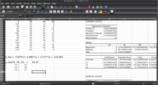
10.1- This model is strong since the significance of F is 1.178E-26, which is ~0 and less than 0.05. The strongest predictor variables are New Cap. Exp. and Value Added By Mfg. since they are the only two variables with p-values less than 0.05. Of the two Value Added By Mfg. is the strongest since it has the smaller p-value.
10.2 – This model is strong since the significance of F is ~0.003 and less than 0.05. The Earnings per Share, Average Yield, and Dividends per Share variables seem to be the best predictors since their p-values are less than 0.05. Out of the three the Earnings per Share variable seems to be the best since its p-value is ~ 0.000047.
10.3 – This model is strong since the significance of F is 7.22E-25 or ~0, which is less than 0.05. The FTSE 100 seems to be the strongest predictor with a p-value of 0.00046. The HANG SENG and IPC are the next best predictors since their p-values are ~0.006. The DIJA is a decent predictor since its p-value is ~0.03 which is less than 0.05. The NASDAQ and S&P 500 would not be considered good predictors of the NIKKEI, since their p-values are significantly greater than 0.05.
10.4- This model is strong since the significance of F is 3.2964E-58 or ~0, which is significantly less than 0.05. The Annual Household income seems to be the strongest predictor since it is 2.29995E-59 or ~0, which is significantly less than 0.05 and Non Mortgage Household Debt ($) is ~0.482 which is significantly larger than 0.05.
